
The role #
From May to August 2026 I worked as an ML Undergraduate Research Assistant at UBC’s Earthquake Engineering Research Facility (EERF), supported by the Work Learn International Undergraduate Research Award (WLIURA), under Mona Amer and Prof. Carlos E. Ventura. The work produced a first-author manuscript now in preparation for Mechanical Systems and Signal Processing.
The project in one sentence: learn the structural dynamics of an operating wind turbine directly from noisy field vibration data, even when rotor harmonics overlap the frequencies we care about.
A spinning machine hides its own structure #
Structural health monitoring leans on a fact: damage changes how a structure vibrates. Natural frequencies shift, damping changes, mode shapes deform. For a quiet civil structure you can estimate those modal properties from response measurements alone, using output-only operational modal analysis (OMA).
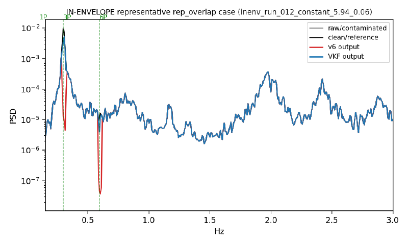
An operating wind turbine breaks the assumptions that make OMA comfortable. The structure is driven by several overlapping sources at once: broadband aerodynamic loading, rotor-synchronous content, blade-passing harmonics, drivetrain and controller effects, and constantly changing rotor speed, wind speed, and operating state. For a three-bladed turbine the prominent harmonics sit at one, three, and six times the rotational frequency (1P, 3P, and 6P), and because rotor speed varies, those components shift and broaden across the spectrum. When one lands on a structural resonance, the operational component can be as strong as, or stronger than, the structural response, and a classical method has trouble deciding whether a peak belongs to the structure or to the rotation.
This matters because the turbines being built in remote, seismically active regions like southwestern British Columbia are expensive to reach. Condition-based maintenance needs a way to watch the structure continuously, during normal operation, without a shutdown. That is the problem this system is designed around.
The data #
The system was developed around real operational measurements from a utility-scale turbine (Cape Scott T22, Vestas-200 class) on Vancouver Island’s north coast, with tower-mounted accelerometers at four heights: 0, 17, 47, and 78 m.
The harmonic-cleaning stage works on the triaxial response: 4 heights times 3 directions, 12 power-spectrum channels. The modal estimator downstream uses the horizontal response: 4 heights times 2 directions, 8 channels organized as a 4-node graph whose layout mirrors the physical ordering of sensors up the tower.
Data are organized into 10-minute windows, and the models consume spectral representations (power spectral density and cross-power spectral density) rather than raw time series. Frequency-domain inputs let the system reason directly about resonance location, damping-controlled peak width, cross-channel coherence, and rotor-harmonic contamination. Simulation corpora from the matching OpenFAST model supply controlled training pairs and benchmarks.
Stage 1: tell the network where rotation should appear #
A naive learned denoiser faces an impossible choice: a large spectral peak might be a rotor harmonic, but it might be a genuine structural resonance. Blindly suppressing large peaks risks deleting the physics you are trying to measure.
The cleaner therefore gets an explicit rotor-derived prior. It combines three ingredients:
- A harmonic comb mask, built from SCADA rotor speed, that marks where 1P, 3P, and 6P energy is expected for this window. The mask localizes harmonic removal to physically plausible regions.
- FiLM conditioning, which feeds operating-state variables (mean rotor speed, within-window spread, amplitude near 1P) into the convolutional backbone so the cleaning strength adapts to the operating condition.
- An attenuation-only residual: the network predicts a correction that is constrained to remove energy, never add it. It cannot invent peaks.
It is not a fixed notch filter; the attenuation pattern changes with the measured spectrum and the operating state. The comb-mask plus FiLM hybrid outperformed purely learned variants in cleaner-specific evaluations, and it was trained on 130 paired OpenFAST cases, each matching a rotating simulation with harmonics against a standstill simulation of the same turbine and wind conditions.
Stage 2: turn the tower into a graph #
After cleaning, the modal estimator represents the instrumented tower as a graph: one node per sensor height, edges along the tower from base to nacelle. Each node starts from a shared spectral encoder that compresses that sensor’s cleaned response into 64 learned features, plus height and operating-condition information. Message passing then lets neighboring tower levels exchange information before the model predicts global modal properties and per-node mode-shape components.
The message passing is deliberately directional. A tower with a clamped base and a nacelle-loaded top is not symmetric along its height, so information travelling up-tower and down-tower passes through separate learned transformations. This was not a cosmetic choice: in the architecture searches, the message-passing operator itself materially changed whether the weaker second modal family was recovered. It became part of the physical inductive bias of the estimator.
Learning without modal labels #
Field vibration data comes with no table of correct frequencies, damping ratios, or mode shapes; that absence is exactly what makes modal identification hard. So the estimator is trained self-supervised: for every window it predicts a small set of candidate modal components, and those parameters must reconstruct the measured cross-spectral density through a conventional modal response model. Training asks one question: if these were really the modes present in the turbine, could they regenerate the measured multi-sensor response?
The decoder is where machine learning meets modal dynamics. Each predicted mode contributes a rank-one cross-spectral term:
Ĝ(f) = Σₖ Aₖ · Lₖ(f; fₖ, ζₖ) · φₖ φₖᴴ + N(f)
where fₖ is the modal frequency, ζₖ the damping ratio, Aₖ the contribution amplitude, φₖ the complex mode shape, Lₖ a resonance profile, and N a diagonal broadband background. The network cannot explain the data with an arbitrary neural tensor; it has to explain it as a small collection of modal systems. Auxiliary label-free losses keep predicted frequencies anchored to actual spectral peaks, smooth across similar operating states, and keep paired slots from collapsing onto the same shape.
Two design choices deserve their own mention:
- Frequency gets its own evidence pathway. Early versions predicted frequency from a globally pooled graph representation and could learn a coarse answer. The final model instead predicts a frequency distribution over an allowed band and refines it around the strongest local evidence, which keeps each slot anchored to the spectrum.
- No prescribed mode shapes. The system deliberately avoids using an analytical Euler-Bernoulli shape as a training target. Analytical shapes and classical estimates are used for interpretation and validation only, so that any shape agreement is discovered from the measurements rather than trained in. An earlier analytical prior improved some shape metrics while making it harder to know whether the model had actually found the shape; it was removed.
Validation needs more than one reference #
There is no perfect table of modal truth for an operating utility-scale turbine, so the work validates from several directions, each answering a different question:
- Synthetic known-truth benchmark: a generator with known frequencies and shapes, including a deliberately weak mode, tests recovery when the answer is known.
- Rotating OpenFAST benchmark: 27 held-out source-disjoint runs with condition-matched linearization references test frequency accuracy under realistic simulated operation.
- Independent field SSI: covariance- and data-driven stochastic subspace identification on raw field windows, plus an adversarial audit (changed thresholds, preprocessing, hour boundaries), tests which field frequency families are reproducible rather than artifacts.
- Matched SSI-CPSD evaluation: window-by-window comparison of neural slot allocation against the SSI families actually present, including leave-one-date-out folds.
- Reproducibility: whether a modal family persists across time windows, random seeds, preprocessing variants, and architecture variants.
A note on wording, which the manuscript takes seriously: an SSI frequency is an independent reference, not ground truth; a neural slot near a reference does not confirm physical mode identity; and simulation is not automatically truth.
Results #
The first bending mode is recovered robustly #
The clearest result is the turbine’s dominant first tower-bending family. Across repeated experiments, model variants, and training seeds, the estimator consistently identifies a low-frequency structural mode in the expected region and recovers a spatial shape in strong agreement with independent classical references: validation records report MAC values above 0.99 for the strongest first-mode cases against independent SVD/SSI references. This matters precisely because the model was never trained on those references; it learns the shape indirectly by reconstructing the measured dynamics.
The weaker mode taught us more than the easy one #
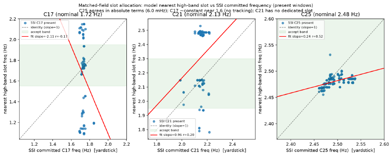
The higher-frequency band was the hard, instructive part. Independent SSI resolved three recurrent frequency families near 1.72, 2.13, and 2.48 Hz, robust to analysis-threshold and preprocessing changes (the 2.48 Hz family appears in essentially every window; its profile resembles an Euler-Bernoulli Mode 2 reference and its frequency sits near the parked OpenFAST eigenfrequency). The families are approximately RPM-flat, which supports a structural interpretation. They also coexist within single hours.
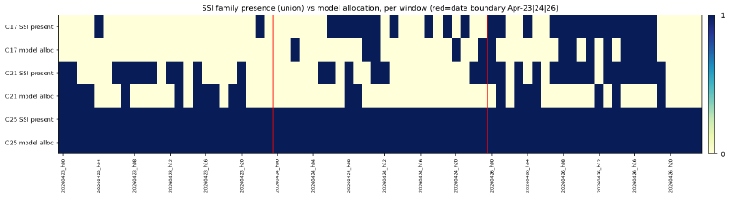
The honest negative result: the current decoder has two high-band slots, and it does not yet allocate them reliably to whichever families coexist in a given window. Fixed and leave-one-date-out trained models settle into dominant fixed-family solutions instead. This capacity and allocation failure is reported as a result, ablated (widened search bands and alternative pooling did not fix it), and used to motivate the next architecture: slot-specific local spectral pooling or attention. A model can reconstruct the measured spectrum well while still choosing the wrong physical decomposition, which is exactly why interpretability and independent references matter here.
Benchmarks: honest comparisons against classical methods #
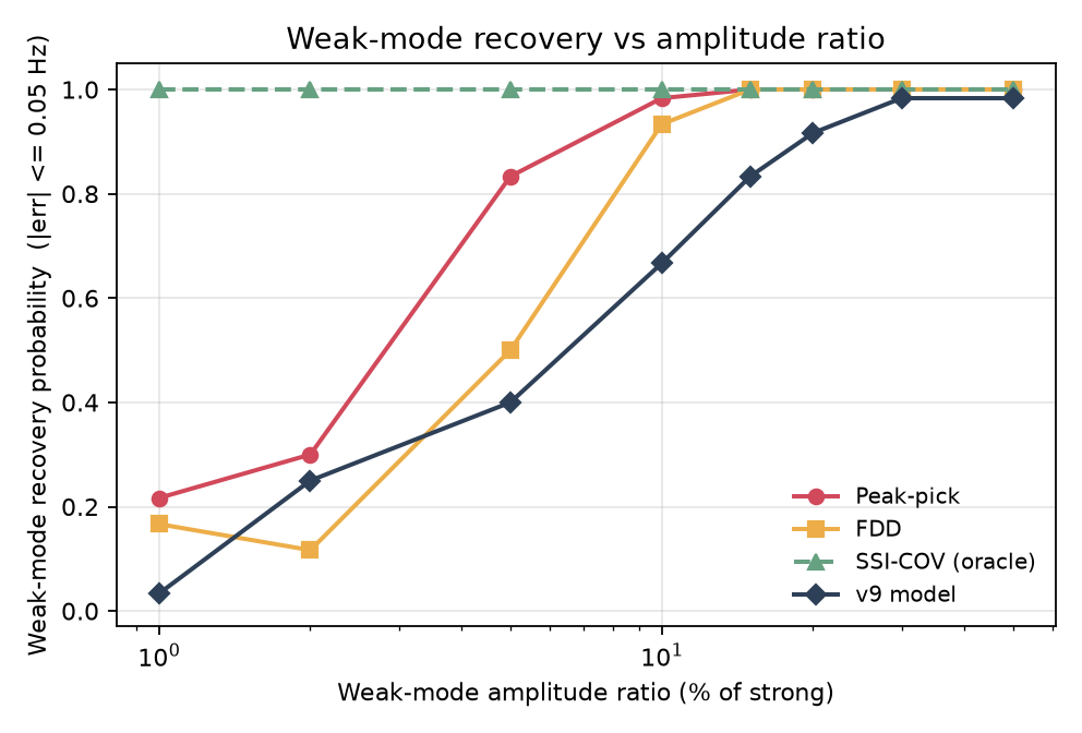
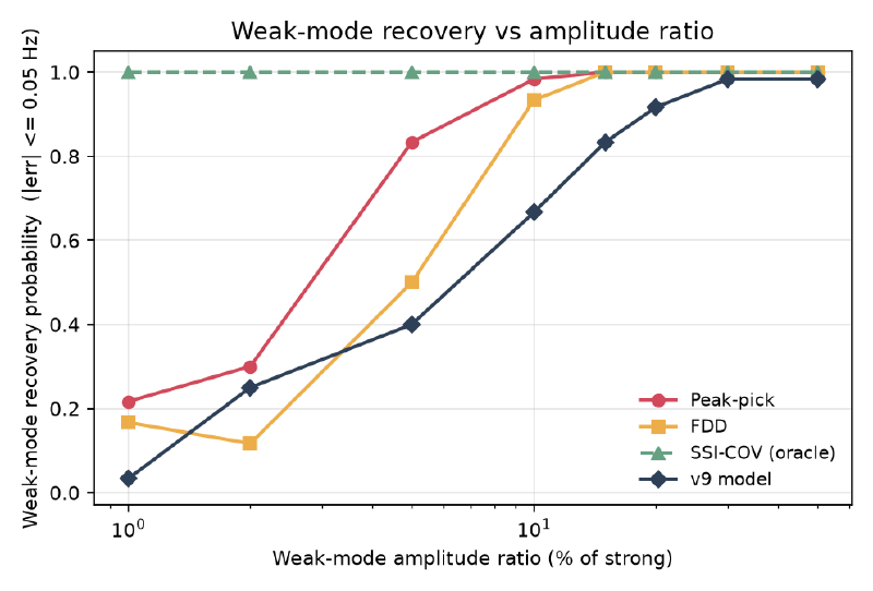
On the synthetic weak-mode test, the graph model cut weak-mode frequency error from 0.246 Hz (FDD) to about 0.035 Hz and raised weak-mode shape agreement (MAC) from 0.13 to about 0.72, while FDD kept the edge on the strong isolated mode.
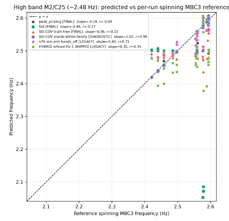
On the 27 held-out rotating OpenFAST cases with condition-matched linearization references, SSI-COV remains the precision estimator:
| Method | Median high-band frequency error |
|---|---|
| SSI-COV (closest stable pole) | 0.00141 Hz |
| FDD | 0.03184 Hz |
| Graph model, best configuration | 0.02813 Hz |
| Peak-picking | 0.05863 Hz |
Once trained, estimation is fast #
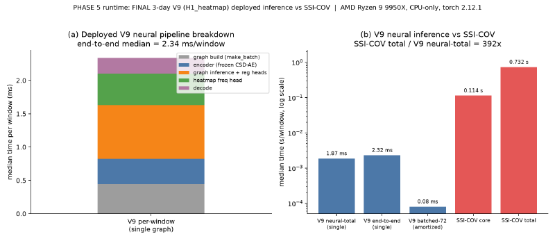
A single neural forward pass takes about 2 ms per window against a median of about 1.4 s per window for the SSI-COV analysis: roughly a 700-fold difference once spectra are prepared, and about a 12-fold wall-time advantage on the practical raw-record path (measured on different hardware classes, RTX 5080 for inference versus CPU workers for SSI). The model’s role is a fast screening and tracking layer for months of continuous data, with SSI as the precision instrument.
What actually mattered #
The ablations taught more than the headline numbers. The lesson was not that more complexity helps; several sophisticated additions failed to improve the physics.
- Message passing matters. The directionally coupled graph layer was selected after a broader architecture search; the operator choice materially affected recovery of the weaker family.
- Narrower, physically plausible search bands helped. Constraining each slot to its relevant spectral region reduced convergence to energetic but physically wrong peaks.
- The analytical shape prior was removed on purpose. It made evaluation look better without proving the model had discovered anything.
- More regularization did not automatically help. Several independence, sparsity, and evidence-gating losses were tested; some improved one metric while hurting the decomposition. The final objective stays comparatively simple.
The bigger goal: monitoring before and after extreme events #
This work sits inside a broader EERF research effort on wind turbines in seismic-prone regions. A future monitoring system has to distinguish ordinary operating variability, wind and rotor-state effects, environmental variability, and true structural change from each other. If a system cannot reliably tell a rotor harmonic from a structural resonance during normal operation, it cannot safely interpret a frequency shift after an earthquake as damage.
The long-term direction: identify modal properties reliably during ordinary operation, track their natural variability, compare pre-event and post-event behavior, connect the field pipeline to controlled shake-table experiments at EERF, and build toward a validated structural model for decision support. This project establishes the modal-identification foundation; it does not yet claim damage classification.
What this does not prove #
- One primary real turbine dataset. The most extensive validation is the Cape Scott corpus; generalization to other turbines, layouts, and environments remains to be demonstrated.
- The second modal family remains harder than the first. Higher-frequency estimates are more sensitive to architecture, band selection, and competing content, and the reported frequency families are strata, not confirmed mode numbers.
- The cleaner is channel-wise. It attenuates harmonic content in per-channel spectra; it does not perform full complex cross-spectral phase denoising.
- Simulation is not automatically truth. OpenFAST supplies controlled experiments and paired training corpora, not certified modal labels for the field structure.
- Identification is not damage classification. The damage-detection goal comes after this foundation is solid.
Where it goes next #
Stronger fully-tuned classical baselines with transparent parameter sweeps; cross-spectral-native harmonic separation that reasons about complex CSD structure rather than channel-wise gains; broader turbine and seasonal validation; uncertainty estimation so the system can say when its evidence is weak; slot-specific local spectral pooling or attention to fix high-band allocation; and shake-table validation at EERF where structural state can be manipulated and independently measured.
Jargon decoder #
Details
- Modal parameters: the natural frequencies, damping ratios, and mode shapes that describe how a structure vibrates, and that shift when it is damaged.
- Operational Modal Analysis (OMA): estimating those parameters from vibration measured during normal operation, with no controlled excitation.
- 1P, 3P, 6P: rotor-synchronous harmonics at one, three, and six times the rotational frequency of a three-bladed turbine.
- PSD / CPSD: power spectral density, and its cross-channel cousin, the cross-power spectral density, which captures how sensor pairs relate in magnitude and phase.
- Comb mask: a smooth mask marking the frequency regions where rotor harmonics are expected for the current rotor speed.
- FiLM: feature-wise linear modulation; conditioning a network so operating-state inputs scale and shift its internal features.
- GNN: graph neural network; here, four nodes representing four sensor heights exchanging information along the tower.
- Modal slot: a candidate dynamical component (frequency, damping, amplitude, shape) that must explain part of the observed spectrum; not a “Mode 1/Mode 2” class label.
- SSI / FDD: stochastic subspace identification and frequency-domain decomposition, the two classical OMA methods used as independent references.
- MAC: modal assurance criterion, a 0 to 1 measure of agreement between two mode shapes.
- Euler-Bernoulli: the classical beam theory whose analytical cantilever shapes serve as reference-only comparisons.
- OpenFAST: the open-source wind turbine simulation code from NREL, used for matched rotating/standstill corpora and controlled benchmarks.
- SCADA: the turbine’s supervisory control and data logs, the source of rotor-speed measurements.
Tools #
- PyTorch and PyTorch Geometric for the harmonic cleaner, shared spectral encoder, and directional graph estimator.
- OpenFAST corpora generation and processing; Welch-based PSD/CPSD pipelines with careful window and unit handling.
- SCADA-to-acceleration alignment, decimation, and calibration for the Cape Scott acquisition system; deployment support for future data collection.
- Multi-seed experiment harness for architecture comparisons and ablations, on CUDA and Slurm.